
CNN for Malware Detection
layout: single title: “Malware Classification with Convolutional Neural Networks” permalink: /projects/malware_classification/ —
In this project, I worked on a deep learning reproduction study focused on malware family classification from binary images. The idea is unusual but powerful: instead of hand-engineering static features from executable files, the raw bytes of malware samples are transformed into grayscale images and classified using a convolutional neural network (CNN).
The project had two main goals. First, we reproduced the CNN architecture proposed in the paper Using convolutional neural networks for classification of malware represented as images. Second, we extended the work through nested cross-validation and hyperparameter tuning, and then evaluated the best architecture on a much larger malware dataset collected beyond the original benchmark.
This project gave me practical experience at the intersection of cybersecurity, computer vision, and model evaluation. It was particularly interesting because the input data was not natural imagery, but executable binary structure represented visually.
The Problem
Malware comes in many forms: trojans, worms, ransomware, spyware, backdoors, downloaders, and other malicious executables. Although these categories are useful at a high level, in practice many datasets organize malware into families, meaning groups of samples that share code structure, behavior, or origin.
Traditional malware analysis often relies on:
- handcrafted static features,
- manual reverse engineering,
- dynamic sandbox execution,
- or signature-based detection.
These approaches can be powerful, but they can also be expensive, slow, or brittle when malware variants change slightly.
This project explored a different idea: can we classify malware directly from its raw binary content by turning it into an image and letting a CNN learn discriminative patterns automatically?
Why Represent Malware as Images?
Executable files are ultimately just sequences of bytes. If those bytes are interpreted as pixel intensities, a binary file can be reshaped into a grayscale image. This image does not look meaningful to a human in the same way as a photograph, but it often preserves structural patterns from the file:
- repeated code or data sections,
- packed or encrypted regions,
- header structure,
- family-specific layout patterns,
- and texture-like artifacts caused by similar compilation or obfuscation methods.
That makes CNNs a natural candidate, since they are good at extracting local spatial patterns and hierarchical features.
In other words, the model is not “seeing” malware semantically like a reverse engineer would. Instead, it is learning statistical visual patterns that correlate with malware families.
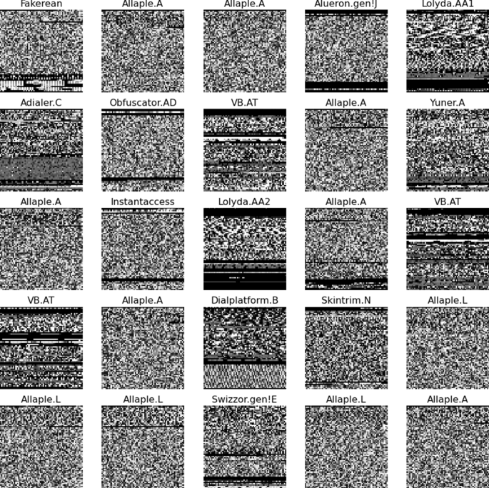
Figures From the Paper
The original article included binary-image examples that show how malware families can look visually distinct once raw bytes are mapped into grayscale.
Try It Yourself: Interactive Binary Visualizer
🔍 Interactive Binary Malware Visualization
Try it yourself: Enter text below to see it transformed into binary and scanned.
Each bit is rendered as a pixel (black=1, white=0)
What We Did
This project was structured as a reproduction-and-extension study.
We:
- reproduced the CNN architecture from the reference paper,
- evaluated it using 10-fold cross-validation on the MalImg dataset,
- implemented nested cross-validation for more reliable hyperparameter tuning,
- searched across multiple CNN architectures,
- selected the best-performing model,
- and then tested that model on a much larger malware-image dataset (~147 GB).
The main objective was not only to match the published results, but also to examine whether a more carefully tuned model could generalize better.
My Contribution
I worked on understanding and implementing the full experimental pipeline, including:
- CNN-based malware image classification,
- reproducible evaluation using cross-validation,
- nested cross-validation for hyperparameter search,
- interpretation of performance across malware families,
- and comparison between benchmark-dataset performance and larger-scale real-world data.
What made this project interesting to me was that it combined rigorous machine learning evaluation with a very unconventional computer vision input representation.
Model Architecture
The baseline model came from the paper we reproduced. On top of that, we explored several alternative CNN architectures by varying:
- the number of convolutional layers,
- the number of feedforward layers,
- the number of output channels,
- the hidden dimensions of dense layers,
- and the convolution kernel sizes.
The search space included architectures with 2, 3, and 4 convolutional layers.
Hyperparameter Grid
| Number of Convolutional Layers | Number of Feed Forward Layers | Number of Output Nodes | FeedForward Layer Output Sizes | Kernel Size for Convolution Layer |
|---|---|---|---|---|
| 2 | [1, 2] | [40, 50], [70, 90] | [25], [50, 25] | [5, 3], [9, 5] |
| 3 | [1, 2] | [25, 50, 50], [50, 70, 70], [70, 90, 90] | [25], [50, 25] | [5, 3, 3], [9, 5, 5] |
| 4 | [1, 2] | [20, 30, 40, 50], [50, 70, 70, 90] | [25], [50, 25] | [5, 3, 3, 3], [9, 5, 5, 3] |
Why Nested Cross-Validation?
A key part of the project was using nested cross-validation rather than only ordinary cross-validation.
Regular cross-validation gives a decent estimate of performance, but when hyperparameters are tuned on the same folds used for evaluation, performance can appear overly optimistic. Nested cross-validation separates these two steps:
- the inner loop performs hyperparameter tuning,
- the outer loop evaluates the tuned model on unseen data.
This gives a more realistic estimate of how well the model architecture actually generalizes.
For a project like this, that mattered a lot: it allowed us to distinguish between a model that simply fit the benchmark well and a model that was genuinely more robust.
Results on the MalImg Dataset
The grid search showed a few clear trends:
- the best-performing architecture had 3 convolutional layers,
- the 2-layer CNN performed nearly as well,
- adding a second feedforward layer generally reduced performance.
Best Parameters Found
| Convolutional Layers | Feed Forward Layers | Output Nodes | Output Sizes | Kernel Size |
|---|---|---|---|---|
| 4 | 1 | [50, 70, 70, 90] | [25] | [5, 3, 3, 3] |
| 3 | 1 | [70, 90, 90] | [25] | [5, 3, 3] |
| 2 | 1 | [40, 50] | [25] | [5, 3] |
Accuracy by Number of Convolutional Layers
| Number of Convolutional Layers | Test Accuracy | Test MAE | Std. Dev. Accuracy | Std. Dev. MAE |
|---|---|---|---|---|
| 4 | 97.27% | 0.30 | 0.151 | 0.017 |
| 3 | 98.62% | 0.07 | 0.149 | 0.004 |
| 2 | 98.52% | 0.07 | 0.084 | 0.009 |
The best model therefore used:
- 3 convolutional layers
- output channels [70, 90, 90]
- kernel sizes [5, 3, 3]
- 1 feedforward layer
This tuned model performed very similarly to the original paper’s architecture overall, but gave us a better understanding of which architectural choices actually mattered.
Confusion Matrices
Paper Baseline Model
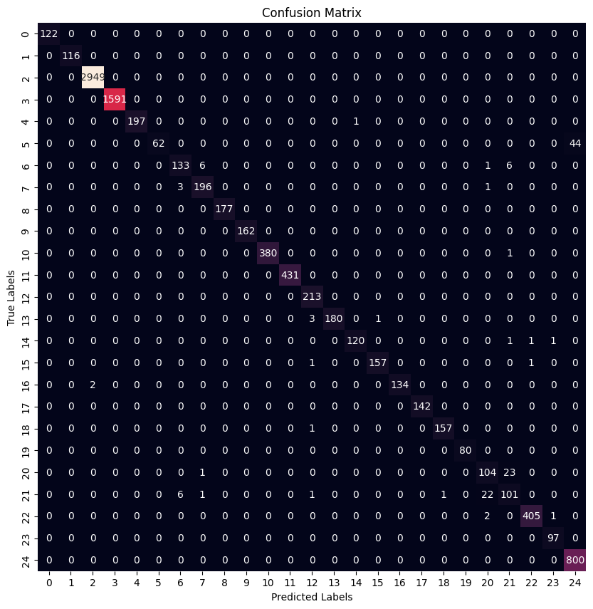
Best Tuned Model

These results show that both models performed very strongly on many malware families, while a smaller subset of classes remained more difficult. This is typical in malware-family classification, where some families are visually and structurally much more distinct than others.
Results on the Larger Dataset
Once we identified the best architecture on MalImg, we tested it on a much larger malware dataset (~147 GB). As expected, performance dropped compared with the smaller benchmark: the classification task became harder because the dataset was larger, more diverse, and less cleanly separable.
Still, the model achieved reasonable performance under 10-fold cross-validation:
| Folds | Accuracy | MAE |
|---|---|---|
| Fold 1 | 89% | 18.68 |
| Fold 2 | 89% | 18.72 |
| Fold 3 | 89% | 19.08 |
| Fold 4 | 90% | 17.50 |
| Fold 5 | 88% | 20.00 |
| Fold 6 | 89% | 18.14 |
| Fold 7 | 89% | 19.20 |
| Fold 8 | 89% | 18.51 |
| Fold 9 | 89% | 18.68 |
| Fold 10 | 89% | 19.45 |
| Average | 89.47% | 18.80 |
| Standard Deviation | 0.447% | 0.657 |
This was an important finding: even though performance dropped from the curated benchmark, the tuned CNN still transferred reasonably well to a much larger and harder dataset.
What I Learned
This project taught me several useful lessons:
- benchmark performance can be misleading without careful evaluation,
- nested cross-validation is worth the extra effort when tuning models,
- unusual data representations can work surprisingly well,
- and strong results on a clean dataset do not always carry over directly to larger real-world data.
More broadly, it showed me how computer vision ideas can be applied far beyond ordinary photographs, including domains like cybersecurity where the “images” are really encoded structure from non-visual data.
Limitations
Although the results were strong, this approach also has limitations.
The model does not truly “understand” malware in a semantic or behavioral sense. It learns visual patterns associated with malware families. That means:
- it may struggle with heavily obfuscated or novel malware,
- it does not replace dynamic or behavioral analysis,
- and strong classification accuracy does not automatically mean production-grade malware detection.
So this project is best understood as a data-driven malware family classifier, rather than a complete antivirus system.
Example: Turning a File into an Image
One of the most interesting ideas in this project is the input transformation itself.
At a high level, the process is:
- take the raw bytes of a binary file,
- interpret each byte as an integer from 0 to 255,
- map those values to grayscale pixels,
- reshape the stream into a 2D image,
- feed the image into a CNN.
For example, a simplified byte sequence like:
4D 5A 90 00 03 00 00 00 FF FF 00 B8