01.

The Problem

Construction stakeout is the process of transferring design points from a digital model onto the physical site. It is typically done with a robotic total station (RTS) tracking a prism mounted on a handheld pole. The achievable accuracy is limited by one frustratingly manual constraint: the operator has to hold the pole perfectly vertical. Any tilt translates into a lateral error at the tip that grows with the pole length.

Keeping the pole level to tolerance is slow and cognitively demanding — the operator iteratively nudges the pole, checks a spirit level, and re-reads the display for every single point. This fine-navigation phase accounts for roughly 25 % of a surveyor’s working time, at around 2–3 minutes per point.

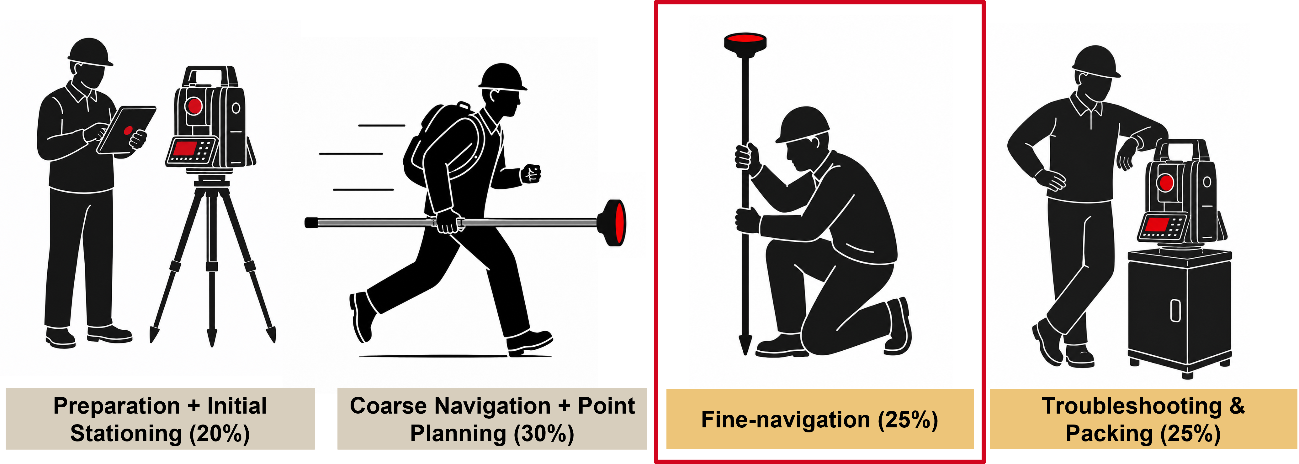
The premise of the thesis: if the pole’s orientation were estimated in real time by fusing the RTS with an inertial measurement unit (IMU), the system could correct for tilt automatically. The levelling cycle disappears, and the operator only has to bring the tip onto the target.

02.

The Approach

Prior work had shown RTS–IMU tilt compensation was possible, but relied on sub-millisecond hardware synchronisation, pre-corrected measurements, and laboratory-calibrated geometry. I set out to reach comparable accuracy under realistic field constraints — no hardware sync, raw instrument measurements, and in-field calibration. That required three contributions:

1. A tilt-aware RTS measurement model. The instrument internally assumes a vertical pole when reporting the prism position. The model corrects for this by folding the estimated pole attitude and prism geometry back into the measurement equation.
2. An in-field lever-arm calibration. When the operator holds the tip fixed and rotates the pole through a range of inclinations, the prism traces the surface of a sphere centred on the fixed tip. From a sequence of such rotations, the unknown IMU-to-tip translation becomes observable — no lab equipment needed.
3. A delay-aware extension. The unknown RTS↔IMU clock offset is treated as an optimisation variable, recovered through piecewise-linear pose interpolation between keyframes.

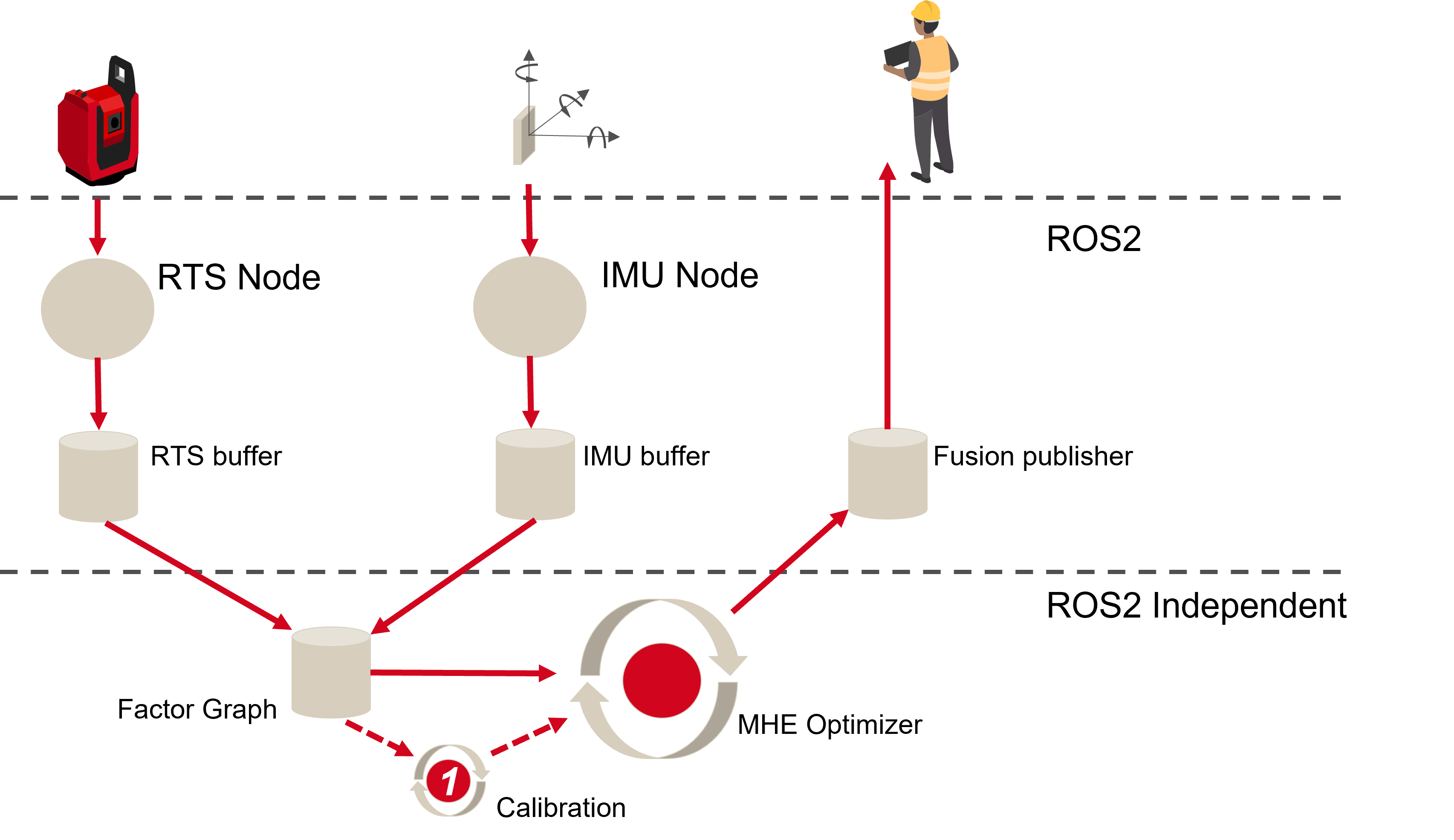
Everything is expressed as a factor graph — each sensor measurement and physical constraint contributes a separate cost term to one joint optimisation. This structure lets the calibration routine reuse the same variables, and lets the estimator revisit past states (which a forward-only filter such as an EKF cannot do).

03.

Estimation: the Moving-Horizon Estimator

A factor graph alone would grow without bound over a long survey. To keep the cost per update fixed, the graph is solved by a moving-horizon estimator (MHE): it optimises over a sliding window of the $N$ most recent keyframes, where each keyframe is aligned with an incoming RTS measurement. As the window advances, the oldest state is marginalised out via the Schur complement and summarised by an arrival cost that carries forward everything that left the window.

The estimator solves, at each step:

where each term is a squared, covariance-weighted residual:

• $\mathbf{r}_{A}(\mathbf{x}_K)$ — the arrival cost, a prior on the first state in the window summarising all marginalised measurements.
• $\mathbf{r}^{\mathrm{IMU}}{k,k+1}$ — the IMU pre-integration factor between consecutive keyframes, weighted by the propagated pre-integration covariance $\boldsymbol{\Sigma}{k,k+1}$.
• $\mathbf{r}{k}$ — the tilt-aware RTS factor, weighted by the fixed RTS measurement covariance $\boldsymbol{\Sigma}{\mathrm{RTS}}$.

The decision variables are the window’s keyframe states $\mathcal{X}_{K:K+N}$ plus a shared parameter block $\mathbf{x}_0$ holding the IMU biases. The marginalisation is handled internally by GTSAM. In the delay-aware variant, $\mathbf{x}_0$ is augmented with the scalar clock-offset $\delta$ and the RTS residual is evaluated on an interpolated pose.

04.

Characterising the Sensors

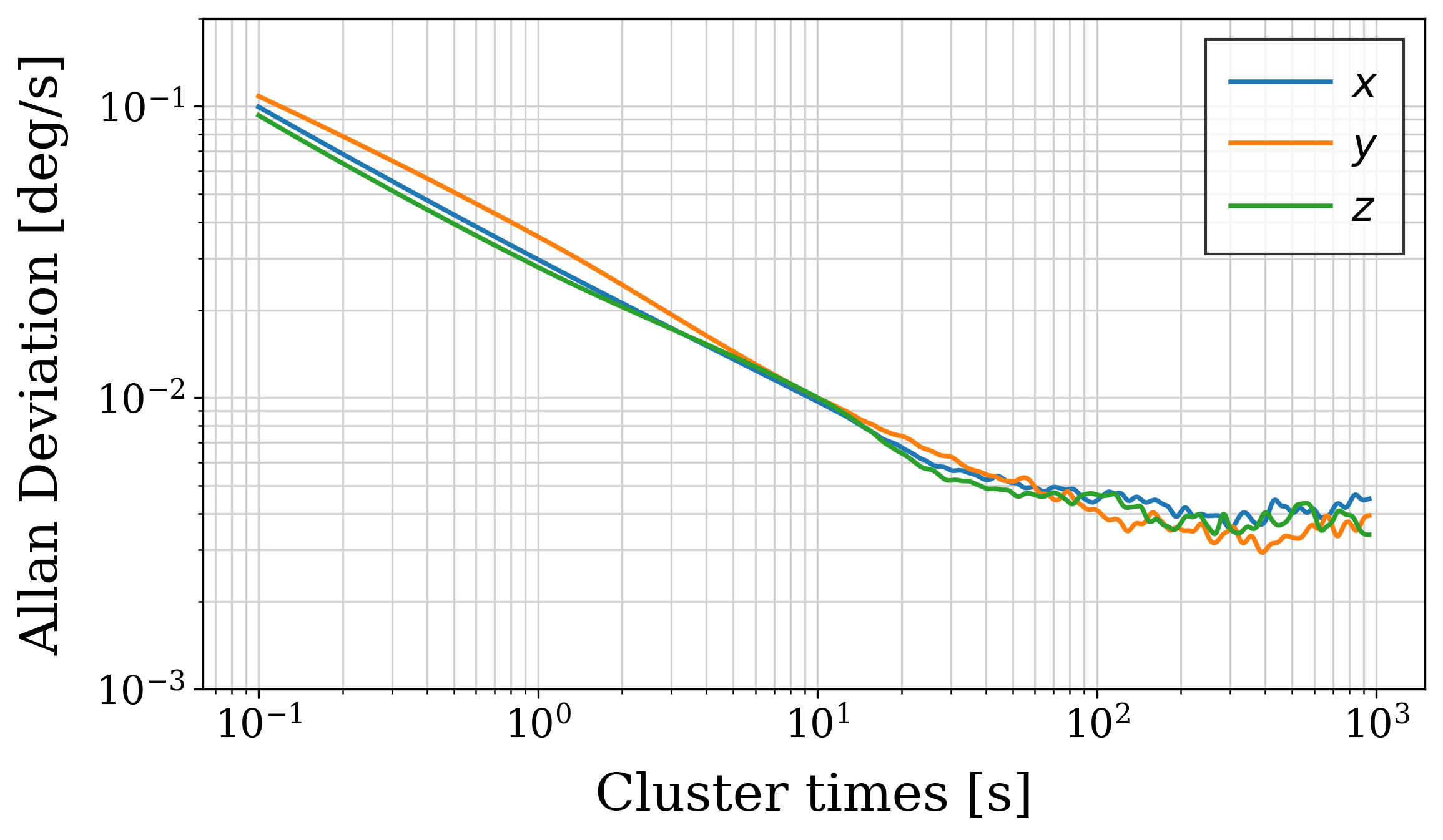
A least-squares estimator is only as good as the covariances you feed it. The IMU noise parameters that set $\boldsymbol{\Sigma}_{k,k+1}$ were determined from an Allan-variance analysis of long static recordings, and the RTS covariance was determined experimentally against an external motion-capture reference.

05.

Results

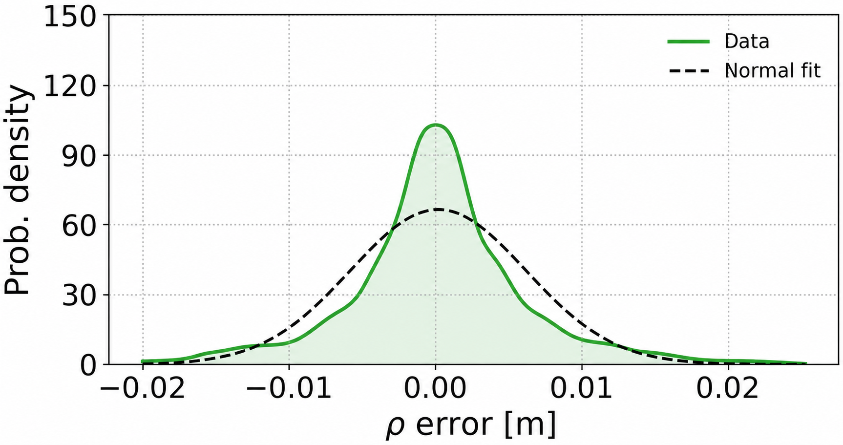
In the fine-navigation regime the MHE reaches a 2D RMSE of about 5.8 mm, meeting the sub-centimetre target despite the absence of hardware synchronisation and a less accurate instrument than prior work. The radial error stays tightly concentrated around zero:

Crucially, the levelling cycle was eliminated: in the experiments, stakeout took under 30 seconds per point instead of 2–3 minutes. Extrapolated across a working day, that would shrink the fine-navigation period from roughly two hours to under thirty minutes.

The dominant remaining error source is calibration uncertainty — the pole tip subtly shifting its contact point during the calibration rotations. Tightening that procedure is the clearest direction for future work.